JDK1.8 HashMap源码简单讲解

JDK1.8 HashMap源码简单讲解

1.成员常量类

1.1 序列化版本号

1
private static final long serialVersionUID = 362498820763181265L;

1.2 集合的初始容量

1
2
3
4
5
/**
* The default initial capacity - MUST be a power of two.
* 默认容量是16,必须是2的n的n次幂
*/
static final int DEFAULT_INITIAL_CAPACITY = 1 << 4; // aka 16

1.2.1 问题:为什么必须是2的n次幂?如果输入值不是2的幂,比如17会怎么样?

这样做是为了减少hash碰撞的次数, 2的n次方实际就是1后面n个0,2的n次方减1二进制表示时实际就是n个1;

按位与运算 : 相同的二进制数位上,都是1的时候,结果为1,否则为零。

按位或运算 : 相同的二进制数位上,都是0的时候,结果为0,否则为1。

1
2
3
4
5
6
7
8
9
10
11
12
13
14
15
16
17
18
19
20
21
22
23
24
25
26
27
28
29
30
31
32
33
34
hash计算存放位置的时候,是通过hash&(length-1)
例如1
hash值如果为3,hashmap默认容量为16 ,即 3 & (16-1)
0000 0011 3
0000 1111 15
------------------
0000 0011 3 索引值为3

例如2
hash值如果为5,hashmap默认容量为16 ,即 5 & (16-1)
0000 0101 5
0000 1111 15
------------------
0000 0101 5 索引值为5

------------------------------------------------
如果不是2的n次幂
hash值如果为3,hashmap容量设置为17 ,即 3 & (17-1)
0000 0011 3
0001 0000 16
------------------
0000 0000 0 索引位置为0

hash值如果为7,hashmap容量设置为17 ,即 7 & (17-1)
0000 0111 7
0001 0000 16
------------------
0000 0000 0 索引位置为0

hash值如果为9,hashmap容量设置为17 ,即 7 & (17-1)
0000 1001 9
0001 0000 16
------------------
0000 0000 0 索引位置为0

总结:

​ 1.由上面可以看出,当我们根据key的hash确定其在数组的位置时, 如果n为2的幂次方,可以保证数据的均匀插入,如果n不是2的幂次方,可能数组的一些位置永远不会插入数据,浪费数组的空间,加大hash冲突。因此,HashMap 容量为2次幂的原因,就是为了数据的的均匀分布,减少hash冲突,毕竟hash冲突越大, 代
表数组中一个链的长度越大,这样的话会降低hashmap的性能

1.2.2 为什么不直接进行取余运算,而是通过位运算

在计算中,数据是采用0101存储的,位运算的效率远比取模%高,所以,使用位运算代替取余操作,来确定元素的存储问题。当前两种方式,得到的结果都是一样的,只是效率不同

1
hash & (length-1)== hash % length

1.2.3 如果初始hashmap的容量不是2的n次幂,会做哪些操作

如果创建HashMap对象时,输入的数组长度是17,不是2的幂,HashMap通过移位运算和或运算得到
的肯定是2的幂次数,并且是离那个数最近的数字。例如如果容量是17,初始化容量就是返回32

下述源码就是初始化时指定大小和负载因子

jdk1.8源码操作如下:

1
2
3
4
5
6
7
8
9
10
11
12
13
14
15
16
17
18
19
20
21
22
23
24
25
26
27
28
29
30
31
32
33
34
35
36
37
38
39
 /**
* Constructs an empty <tt>HashMap</tt> with the specified initial
* capacity and load factor.
*
* @param initialCapacity the initial capacity
* @param loadFactor the load factor
* @throws IllegalArgumentException if the initial capacity is negative
* or the load factor is nonpositive
*/
public HashMap(int initialCapacity, float loadFactor) {
// 如果初始容量小于0,抛出异常
if (initialCapacity < 0)
throw new IllegalArgumentException("Illegal initial capacity: " +
initialCapacity);
// 如果初始容量大于最大容量2^30,复制为最大容量。防止溢出
if (initialCapacity > MAXIMUM_CAPACITY)
initialCapacity = MAXIMUM_CAPACITY;
// 负载因子小于0,报错提示
if (loadFactor <= 0 || Float.isNaN(loadFactor))
throw new IllegalArgumentException("Illegal load factor: " +
loadFactor);
this.loadFactor = loadFactor;
// threshold hashmap扩容阈值,注意这个值会发生变化。
this.threshold = tableSizeFor(initialCapacity);
}

/**
* 返回给定目标容量的2次幂大小。
* Returns a power of two size for the given target capacity.
*/
static final int tableSizeFor(int cap) {
int n = cap - 1;
n |= n >>> 1;
n |= n >>> 2;
n |= n >>> 4;
n |= n >>> 8;
n |= n >>> 16;
return (n < 0) ? 1 : (n >= MAXIMUM_CAPACITY) ? MAXIMUM_CAPACITY : n + 1;
}

上述代码第二个方法,就是操作

说明:
由此可以看到,当在实例化HashMap实例时, 如果给定了initialCapacity(假设是17),由于HashMap的capacity必须都是2的幂次方,因此这个方法用于找到大于等于initialCapacity(假设是17)的最小的2的幂(initialCapacity如果就是2的幂次方,比如说16,则返回的还是这个数)。

下面分析这段源码算法:

a.首先,为什么要对cap做减1操作
1
int n = cap - 1

如果cap已经是2的幂,此时又没有执行这个减1操作, 则执行完后面的几条无符号右移操作之后,返回的capacity将是这个cap的2倍。

注意:

按位与运算 : 相同的二进制数位上,都是1的时候,结果为1,否则为零。

按位或运算 : 相同的二进制数位上,都是0的时候,结果为0,否则为1。

b.下面看看这几个无符号右移操作是干什么的 1是负数 0正数

第一种情况,容量传递的是0

​ 如果n这时为0了(经过了cap-1之后) , 则经过后面的几次无符号右移依然是0,最后返回的capacity是1

​ **第二种情况,n不等于0 **

1
2
3
4
5
6
7
8
9
10
11
12
13
14
15
16
17
18
19
20
21
22
23
24
25
26
27
28
29
30
31
32
33
34
HashMap <String,Object> hashmap = new HashMap<>(17);
cap = 17
int n = cap - 1 = 16;
第一次无符号右移一位
0000 0000 0000 0000 0000 0000 0001 0000 n=16
0000 0000 0000 0000 0000 0000 0000 1000 n >>> 1
------------------------------------------------------
0000 0000 0000 0000 0000 0000 0001 1000 24 ===>n

第二次无符号右移2
0000 0000 0000 0000 0000 0000 0001 1000 n=24
0000 0000 0000 0000 0000 0000 0000 0110 n >>> 2
------------------------------------------------------
0000 0000 0000 0000 0000 0000 0001 1110 n = 30

第三次无符号右移4
0000 0000 0000 0000 0000 0000 0001 1110 n = 30
0000 0000 0000 0000 0000 0000 0000 0001 n >>> 4
------------------------------------------------------
0000 0000 0000 0000 0000 0000 0001 1111 n = 31

第四次无符号右移8
0000 0000 0000 0000 0000 0000 0001 1111 n=31
0000 0000 0000 0000 0000 0000 0000 0000 n >>> 8
-------------------------------------------------------
0000 0000 0000 0000 0000 0000 0001 1111 n=31

第五次无符号右移16
0000 0000 0000 0000 0000 0000 0001 1111 n=31
0000 0000 0000 0000 0000 0000 0000 0000 n >>> 16
-------------------------------------------------------
0000 0000 0000 0000 0000 0000 0001 1111 n=31
执行最后一行代码操作,n>0且小于最大容量,返回31+1 = 32
return (n < 0) ? 1 : (n >= MAXIMUM_CAPACITY) ? MAXIMUM_CAPACITY : n + 1;

Hashmap最大容量的移动位置操作

1
2
3
4
5
6
7
8
9
10
11
12
13
14
15
16
17
18
19
0010 0000 0000 0000 0000 0000 0000 0000 2^30
int n = cap-1;
0001 1111 1111 1111 1111 1111 1111 1111 n=2^30 -1
0000 1111 1111 1111 1111 1111 1111 1111 n >>> 1
-------------------------------------------
0001 1111 1111 1111 1111 1111 1111 1111 2^29


0001 1111 1111 1111 1111 1111 1111 1111 2^29
0000 0111 1111 1111 1111 1111 1111 1111 n>>>2
------------------------------------------------
0001 1111 1111 1111 1111 1111 1111 1111 2^29

.....

最后得到的值一定为
0001 1111 1111 1111 1111 1111 1111 1111 2^29
加一操作后为
0010 0000 0000 0000 0000 0000 0000 0000 2^30

** 总结** :如果容量大于MAXIMUM_CAPACITY 则取最大容量。不到2^30 的容量,通过移位操作后,会得到大于值的最小2的幂。如果当前值就是2的幂次方,返回当前值

1.3 负载因子

1
2
3
4
5
/**
* 负载因子
* The load factor used when none specified in constructor.
*/
static final float DEFAULT_LOAD_FACTOR = 0.75f;

对于负载因子,如果没有特别需求,不要轻易进行更改,因为 JDK 自身的默认负载因子是非常符合通用场景的需求的(逼哥讲过大量研究得出)。如果确实需要调整,建议不要设置超过 0.75 的数值,因为会显著增加冲突,降低 HashMap 的性能。如果使用太小的负载因子,可能会导致更加频繁的扩容,增加无谓的开销,本身访问性能也会受影响。

  • loadFactor越趋近于1,那么数组中存放的数据(entry)也就越多,也就越密,也就是会让链表的长度增加。

  • loadFactor越小,也就是趋近于0,数组中存放的数据(entry)也就越少,也就越稀疏。

如果希望链表尽可能少些。要提前扩容,有的数组空间有可能一-直没有存储数据。加载因子尽可能小一些。
举例:
1.加载因子是0.5。那么16 * 0.5 = 8 如果数组中满8个空间就扩容,这样会造成数组利用率太低了。
2.加载因子是0.9。那么16 * 0.9=14 如果数组中满14个空间就扩容,hash碰撞次数大大增加,那么这样就会导致链表有点多了。导致查找元素效率低。

所以既兼顾数组利用率又考虑链表长度不要太多,经过逼哥 大量测试0.75是最佳方案。

1.4 链表转红黑树的阈值8

1
2
3
4
5
6
7
8
9
/**
* The bin count threshold for using a tree rather than list for a
* bin. Bins are converted to trees when adding an element to a
* bin with at least this many nodes. The value must be greater
* than 2 and should be at least 8 to mesh with assumptions in
* tree removal about conversion back to plain bins upon
* shrinkage.
*/
static final int TREEIFY_THRESHOLD = 8;

问题1: 为什么Map桶中的节点个数要超过8才转红黑树

源码注释中有这么一段描述

1
2
3
4
5
6
7
8
9
10
11
12
13
14
15
16
17
18
19
20
21
22
23
24
25
26
27
28
29
30
31
32
33
34
    * Because TreeNodes are about twice the size of regular nodes, we
* use them only when bins contain enough nodes to warrant use
* (see TREEIFY_THRESHOLD). And when they become too small (due to
* removal or resizing) they are converted back to plain bins. In
* usages with well-distributed user hashCodes, tree bins are
* rarely used. Ideally, under random hashCodes, the frequency of
* nodes in bins follows a Poisson distribution
* (http://en.wikipedia.org/wiki/Poisson_distribution) with a
* parameter of about 0.5 on average for the default resizing
* threshold of 0.75, although with a large variance because of
* resizing granularity. Ignoring variance, the expected
* occurrences of list size k are (exp(-0.5) * pow(0.5, k) /
* factorial(k)). The first values are:
因为树节点的大小大约是普通节点的两倍,所以我们只在bin包含足够的节点时才使用树节点(参见
TREEIFY_THRESHOLD)。当它们变得太小(由于删除或调整大小)时,就会被转换回普通的桶。在使用分布良好的用户
hashcode时,很少使用树箱。理想情况下,在随机哈希码下,箱子中节点的频率服从泊松分布
(http://en.wikipedia. org/wiki/Poisson. distr ibution),默认调整阈值为0.75,平均参数约为0.5,尽管由于调整粒度的差异很大。忽略方差,列表大小k的预期出现次数是(exp(-0.5)*pow(0.5,k)/factorial(k)).

*
* 0: 0.60653066
* 1: 0.30326533
* 2: 0.07581633
* 3: 0.01263606
* 4: 0.00157952
* 5: 0.00015795
* 6: 0.00001316
* 7: 0.00000094
* 8: 0.00000006
* more: less than 1 in ten million
*
* The root of a tree bin is normally its first node. However,
* sometimes (currently only upon Iterator.remove), the root might
* be elsewhere, but can be recovered following parent links
* (method TreeNode.root()).

说明:

1.TreeNodes占用空间是普通Nodes的两倍,所以只有当bin包含足够多的节点时才会转成TreeNodes,而是否足够
多就是由TREEIFY_THRESHOLD(8)的值决定的。当bin中节点数变少时, 又会转成普通的bin。并且我们查看源码的时候发现,链表长度达到8(桶的数量要大于64)就转成红黑树,当长度降到6就转成普通bin.这样就解释了为什么不是一开始就将其转换为TreeNodes, 而是需要一定节点数才转为TreeNodes, 说白了就是权衡,空间和时间的权衡。

2.当hashCode离散性很好的时候,树型bin用到的概率非常小,因为数据均匀分布在每个bin中,几乎不会有bin中链表长度会达到阈值。但是在随机hashCode下,离散性可能会变差,然而JDK又不能阻止用户实现这种不好的hash算法,因此就可能导致不均匀的数据分布。不过理想情况下随机hashCode算法下所有bin中节点的分布频率会遵循泊松分布,我们可以看到,一个bin中链表长度达到8个元素的概率为0.00000006. 几乎是不
可能事件。所以,之所以选择8,不是随便决定的,而是根据概率统计决定的。

也就是说:选择8因为符合泊松分布,超过8的时候,概率已经非常小了,所以我们选择8这个数字。

3.泊松分布

图片原文链接:

http://www.ruanyifeng.com/blog/2015/06/poisson-distribution.html

问题2:基于JDK1.8,hashmap引入了红黑树,为什么一开始不按照红黑树存储。要等到链表长度大于8才转换

​ JDK 1.8以前HashMap的实现是数组+链表,即使哈希函数取得再好,也很难达到元素百分百均匀分布。当HashMap中有大量的元素都存放到同一个桶中时,这个桶下有一条长长的链表, 这个时候HashMap就相当于一
个单链表,假如单链表有n个元素,遍历的时间复杂度就是O(n),完全失去了它的优势。针对这种情况,JDK 1.8
中引入了红黑树(查找时间复杂度为O(logn))来优化这个问题。当链表长度很小的时候, 即使遍历,速度也非
常快,但是当链表长度不断变长,肯定会对查询性能有一定的影响, 所以才需要转成树。

2.TreeNodes占用空间是普通Nodes的两倍,当元素较少时,增加多余的开销

1.5 红黑树退化为链表的阈值

1
2
3
4
5
6
7
/**
* The bin count threshold for untreeifying a (split) bin during a
* resize operation. Should be less than TREEIFY_THRESHOLD, and at
* most 6 to mesh with shrinkage detection under removal.
当桶(bucket) 上的结点数小于这个值时树转链表
*/
static final int UNTREEIFY_THRESHOLD = 6;

1.6 链表转红黑树时,数组的长度最小值

1
2
3
4
5
6
7
/**
* The smallest table capacity for which bins may be treeified.
* (Otherwise the table is resized if too many nodes in a bin.)
* Should be at least 4 * TREEIFY_THRESHOLD to avoid conflicts
* between resizing and treeification thresholds.
*/
static final int MIN_TREEIFY_CAPACITY = 64;

1.7 table 用来初始化

table必须是2的幂

1
2
3
4
5
6
7
/**
* The table, initialized on first use, and resized as
* necessary. When allocated, length is always a power of two.
* (We also tolerate length zero in some operations to allow
* bootstrapping mechanics that are currently not needed.)
*/
transient Node<K,V>[] table;

jdk8之前数组类型是Entry<K,V>类型。从jdk1.8之后是Node<K,V>类型。 都实现了一样的接口:Map.Entry<K,V>.负责存储键值对数据的。在jdk8以后的构造方法中,并没有对table这个成员变量进行初始化,tabl e的初始化被推
迟到了put方法中

1.8 存放元素缓存

1
2
3
4
5
/**
* Holds cached entrySet(). Note that AbstractMap fields are used
* for keySet() and values().
*/
transient Set<Map.Entry<K,V>> entrySet;

1.9 HashMap元素的个数

1
2
3
4
/**
* The number of key-value mappings contained in this map.
*/
transient int size;

1.10 用来记录HashMap的修改次数

1
2
3
4
5
6
7
8
9
/**
* The number of times this HashMap has been structurally modified
* Structural modifications are those that change the number of mappings in
* the HashMap or otherwise modify its internal structure (e.g.,
* rehash). This field is used to make iterators on Collection-views of
* the HashMap fail-fast. (See ConcurrentModificationException).
结构修改是指改变HashMap中的映射数量或修改其内部结构(例如,rehash)
*/
transient int modCount;

1.11 要调整大小的下一个大小值(容量*负载系数)

1
2
3
4
5
6
7
8
9
10
/**
* The next size value at which to resize (capacity * load factor).
* 要调整大小的下一个大小值(容量*负载系数)。 数组长度唱过临界值时会进行扩容操作
* @serial
*/
// (The javadoc description is true upon serialization.
// Additionally, if the table array has not been allocated, this
// field holds the initial array capacity, or zero signifying
// DEFAULT_INITIAL_CAPACITY.)
int threshold;

1.12 解决hash冲突的常用方法有

1.开放定址法
基本思想是:当关键字key的哈希地址p=H(key)出现冲突时,以p为基础,产生另一个哈希地址p1,如果p1仍然冲突,再以p为基础,产生另一个哈希地址p2,…,直到找出一个不冲突的哈希地址pi ,将相应元素存入其中。

2.再哈希法
这种方法是同时构造多个不同的哈希函数:
Hi=RH1(key) i=1,2,…,k
当哈希地址Hi=RH1(key)发生冲突时,再计算Hi=RH2(key)……,直到冲突不再产生。这种方法不易产生聚集,但增加了计算时间。

3.链地址法
这种方法的基本思想是将所有哈希地址为i的元素构成一个称为同义词链的单链表,并将单链表的头指针存在哈希表的第i个单元中,因而查找、插入和删除主要在同义词链中进行。链地址法适用于经常进行插入和删除的情况。

hashmap解决hash冲突就是采用链地址法

4.建立公共溢出区
这种方法的基本思想是:将哈希表分为基本表和溢出表两部分,凡是和基本表发生冲突的元素,一律填入溢出表。

2.hashmap的方法介绍

Node节点

1
2
3
4
5
6
7
8
9
10
11
12
13
14
15
16
17
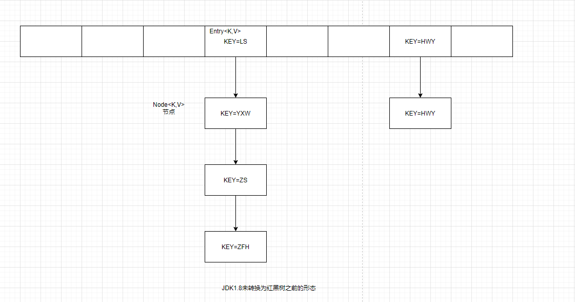
/**
* Basic hash bin node, used for most entries. (See below for
* TreeNode subclass, and in LinkedHashMap for its Entry subclass.)
*/
static class Node<K,V> implements Map.Entry<K,V> {
final int hash;
final K key;
V value;
Node<K,V> next;

Node(int hash, K key, V value, Node<K,V> next) {
this.hash = hash;
this.key = key;
this.value = value;
this.next = next;
}

TreeNode节点部分源码如下:

1
2
3
4
5
6
7
8
9
10
11
12
13
14
15
16
17
18
19
20
21
22
23
24
25
/**
* Entry for Tree bins. Extends LinkedHashMap.Entry (which in turn
* extends Node) so can be used as extension of either regular or
* linked node.
*/
static final class TreeNode<K,V> extends LinkedHashMap.Entry<K,V> {
TreeNode<K,V> parent; // red-black tree links
TreeNode<K,V> left;
TreeNode<K,V> right;
TreeNode<K,V> prev; // needed to unlink next upon deletion
boolean red;
TreeNode(int hash, K key, V val, Node<K,V> next) {
super(hash, key, val, next);
}

/**
* Returns root of tree containing this node.
*/
final TreeNode<K,V> root() {
for (TreeNode<K,V> r = this, p;;) {
if ((p = r.parent) == null)
return r;
r = p;
}
}

2.1 hash值计算方法 hash()

jdk1.8 源码如下:

1
2
3
4
5
6
7
8
9
10
11
12
13
14
15
16
17
18
19
20
21
22
/**
* 计算hash值的方法
* Computes key.hashCode() and spreads (XORs) higher bits of hash
* to lower. Because the table uses power-of-two masking, sets of
* hashes that vary only in bits above the current mask will
* always collide. (Among known examples are sets of Float keys
* holding consecutive whole numbers in small tables.) So we
* apply a transform that spreads the impact of higher bits
* downward. There is a tradeoff between speed, utility, and
* quality of bit-spreading. Because many common sets of hashes
* are already reasonably distributed (so don't benefit from
* spreading), and because we use trees to handle large sets of
* collisions in bins, we just XOR some shifted bits in the
* cheapest possible way to reduce systematic lossage, as well as
* to incorporate impact of the highest bits that would otherwise
* never be used in index calculations because of table bounds.
计算 key.hashCode() 并将散列的较高位(异或)传播到较低位。由于该表使用二次幂掩码,因此仅在当前 掩码之上位变化的散列集将始终发生冲突。 (众所周知的例子是在小表中保存连续整数的浮点键集。)所以我们应用一个变换,将高位的影响向下传播。位扩展的速度、效用和质量之间存在折衷。因为许多常见的散列集已经合理分布(因此不会从扩展中受益),并且因为我们使用树来处理 bin 中的大量冲突,所以我们只是以最便宜的方式对一些移位的位进行异或以减少系统损失,以及合并最高位的影响,否则由于表边界而永远不会在索引计算中使用。
*/
static final int hash(Object key) {
int h;
return (key == null) ? 0 : (h = key.hashCode()) ^ (h >>> 16);
}

我们先研究下key的哈希值是如何计算出来的。key的哈希值是通过上述方法计算出来的。

可以看到当key等于null的时候也是有哈希值的,返回的是0.

这个哈希方法首先计算出key的hashCode赋值给h,然后与h无符号右移16位后的二进制进行按位异或得到最后的
hash值。计算过程如下所示:

1
(h = key.hashCode()) ^ (h >>> 16);

这里其实就是把得到的hashcode转化为32位二进制,然后他的高16位和低16位做了一个异或的操作

举个例子如下:

1
2
3
4
5
6
7
8
9
10
11
12
13
14
15
16
17
18
19
20
21
22
23
24
25
& (按位与运算) : 运算规则:相同的二进制数位上,都是1的时候,结果为1,否则为零。
^ (按位异或运算) :运算规则:相同的二进制数位上,数字相同,结果为0,不同为1.
代码中通过这个hash & (n-1) 得到存储元素的位置
p = tab[i = (n - 1) & hash]

(h = key.hashCode()) ^ (h >>> 16);
假设这里的h = key.hashCode()得到的值为
1111 1111 1111 1111 0000 0000 1111 1111 h
0000 0000 0000 0000 1111 1111 1111 1111 h >>> 16
----------------------------------------------------------
1111 1111 1111 1111 1111 1111 0000 0000 按位异或运算后得到的hash值

此时数据长度n假设为默认的16,那么这个key存放在table中位置为i = (n - 1) & hash
1111 1111 1111 1111 1111 1111 0000 0000 hash
0000 0000 0000 0000 0000 0000 0000 1111 n-1 15 &运算
----------------------------------------------------------
0000 0000 0000 0000 0000 0000 0000 0000 索引位置为0

在存储一个key,假设key的hashcode高位变化较大
1000 1000 0001 0000 1111 1111 0000 0000 hash值
0000 0000 0000 0000 0000 0000 0000 1111 n-1 15 &运算
-------------------------------------------------------
0000 0000 0000 0000 0000 0000 0000 0000 索引位置为0


如果当n的值,即数组长度很小时,假设是默认的16的话,这样的值和hashCode()直接做按位与操作,实际上只使用了哈希值的后4位。如果当哈希值的高位变化很大,低位变化很小,这样就很容易造成哈希冲突了,所以这里把高低位都利用起来,从而解决了这个问题。也是一种为了降低hash冲突的优化手段

​ 为什么这里需要将高位数据移位到低位进行异或运算呢?这是因为有些数据计算出的哈希值差异主要在高位,而 HashMap 里的哈希寻址是忽略容量以上的高位的,那么这种处理就可以有效避免类似情况下的哈希碰撞。

2.2 hashmap的put()方法

1
2
3
4
5
6
7
8
9
10
11
12
13
14
15
16
17
18
19
20
21
22
23
24
25
26
27
28
29
30
31
32
33
34
35
36
37
38
39
40
41
42
43
44
45
46
47
48
49
50
51
52
53
54
55
56
57
58
59
60
61
62
63
64
65
66
67
68
69
70
71
72
73
74
75
76
77
78
79
80
/**
* Associates the specified value with the specified key in this map.
* If the map previously contained a mapping for the key, the old
* value is replaced.
*
* @param key key with which the specified value is to be associated
* @param value value to be associated with the specified key
* @return the previous value associated with <tt>key</tt>, or
* <tt>null</tt> if there was no mapping for <tt>key</tt>.
* (A <tt>null</tt> return can also indicate that the map
* previously associated <tt>null</tt> with <tt>key</tt>.)
*/
public V put(K key, V value) {
return putVal(hash(key), key, value, false, true);
}

/**
* Implements Map.put and related methods.
*
* @param hash hash for key
* @param key the key
* @param value the value to put
* @param onlyIfAbsent if true, don't change existing value 如果为true表示不更改现有的值
* @param evict if false, the table is in creation mode. 表示table为创建状态
* @return previous value, or null if none
*/
final V putVal(int hash, K key, V value, boolean onlyIfAbsent,
boolean evict) {
// p表示当前的节点。n表示表的长度
Node<K,V>[] tab; Node<K,V> p; int n, i;
// hashmap的table表的初始化操作,是在这里进行的。第一次执行的时候,会先在这里进行初始化操作
if ((tab = table) == null || (n = tab.length) == 0)
n = (tab = resize()).length;
// 通过上述hash()方法得到hash值和数组长度进行按位与运算,得到元素的存储位置,如果table表的位置为空,就直接进行存储操作
if ((p = tab[i = (n - 1) & hash]) == null)
tab[i] = newNode(hash, key, value, null);
else {
// 产生了hash碰撞,走下述代码
Node<K,V> e; K k;
// 这里的p的值是上面p = tab[i = (n - 1) & hash ,if语句体虽然没有执行,但是这一段代码是否执行的,判断hash值和key值
if (p.hash == hash &&
((k = p.key) == key || (key != null && key.equals(k))))
e = p;
// 判断当前table中的p节点是不是树节点
else if (p instanceof TreeNode)
e = ((TreeNode<K,V>)p).putTreeVal(this, tab, hash, key, value);
else {
// 遍历链表的,取下一个位置存放新增的元素,这里采用的是尾插法,a.横竖都要遍历链表的长度是否大于树化的阈值,所以遍历的过程中,就直接插入元素了b.可能的因素就是遍历的过程中要比较key值是否相同,和jdk1.7有些不同
for (int binCount = 0; ; ++binCount) {
//如果下一个位置为空,就直接连接在链表后面
if ((e = p.next) == null) {
p.next = newNode(hash, key, value, null);
// 如果链表的长度大于8个时,就进行链表转红黑树的操作
if (binCount >= TREEIFY_THRESHOLD - 1) // -1 for 1st
treeifyBin(tab, hash);
break;
}
// 如果链表的下一个元素不为空,比较hash值和key值
if (e.hash == hash &&
((k = e.key) == key || (key != null && key.equals(k))))
break;
p = e;
}
}
// key值存在,就替换value值。新插入的元素的value值,替换原来这个key的value值
if (e != null) { // existing mapping for key
V oldValue = e.value;
if (!onlyIfAbsent || oldValue == null)
e.value = value;
afterNodeAccess(e);
return oldValue;
}
}
++modCount;
// hashmap的键值对个数大于扩容的阈值,就进行扩容操作
if (++size > threshold)
resize();
afterNodeInsertion(evict);
return null;
}

如图示:桶长度(bucket) 为8的数组

2.5 TreeifyBin()

1
2
3
4
5
6
7
8
9
10
11
12
13
14
15
16
17
18
19
20
21
22
23
24
25
26
27
28
29
30
31
32
33
34
35
36
37
38
39
/**
* Replaces all linked nodes in bin at index for given hash unless
* table is too small, in which case resizes instead.
替换指定哈希表的索引桶中所有的连接节点,除非表太小,否则将修改大小
*/
final void treeifyBin(Node<K,V>[] tab, int hash) {
int n, index; Node<K,V> e;
/* 如果元素数组为空 或者 数组长度小于 树结构化的最小阈值(MIN_TREEIFY_CAPACITY=64) ,就进行扩容操作.对于这个值可以理解为:如果元素数组长度小于这个值,没有必要去进行结构转换.目的是
如果数组很小,那么转红黑树,遍历效率要低一些,这时进行扩容操作,重新计算哈希值,链表的长度有可能就变短了。数据会放入到数组中,这样相对来说效率会高一些
*/
if (tab == null || (n = tab.length) < MIN_TREEIFY_CAPACITY)
resize();
//如果元素数组长度已经大于等于了 MIN_TREEIFY_CAPACITY,那么就有必要进行结构转换了
// 根据hash值和数组长度进行取模运算后,得到链表的首节点
else if ((e = tab[index = (n - 1) & hash]) != null) {
//定义几个变量,hd代表头节点,tl代表尾节点
TreeNode<K,V> hd = null, tl = null;
do {
//先把e节点转成TreeNode类型,并赋值给p
TreeNode<K,V> p = replacementTreeNode(e, null);
//如果尾节点tl为空,则说明还没有根节点,试想下,这时元素数目都超过8个了,还能没有尾节点么,所以没有尾节点只能说明还没设置根节点
if (tl == null)
//设置根节点,把p赋值给根节点hd
hd = p;
else {
//把tl设置为p的前一节点
p.prev = tl;
//把p设置为tl的后继节点,这两步其实就是我指向你,你指向我的关系,为了形成双向链表
tl.next = p;
}
//把首节点设置成p后,把p赋值给尾节点tl,然后会再取链表的下一个节点,转成TreeNode类型后再赋值给p,如此循环
tl = p;
//取下一个节点,直到下一个节点为空,也就代表这链表遍历好了
} while ((e = e.next) != null);
//用新生成的双向链表替代旧的单向链表,其实就是把这个数组对应的位置重新赋值成新双向链表的首节点
if ((tab[index] = hd) != null)
hd.treeify(tab);
}
}

bin 的数量大于 TREEIFY_THRESHOLD 时:如果容量小于 MIN_TREEIFY_CAPACITY,只会进行简单的扩容。如果容量大于 MIN_TREEIFY_CAPACITY ,则会进行树化改造。

本质上这是个安全问题。因为在元素放置过程中,如果一个对象哈希冲突,都被放置到同一个桶里,则会形成一个链表,我们知道链表查询是线性的,会严重影响存取的性能。

最后一行才是转红黑树的操作

2.6 Treeify()

1
2
3
4
5
6
7
8
9
10
11
12
13
14
15
16
17
18
19
20
21
22
23
24
25
26
27
28
29
30
31
32
33
34
35
36
37
38
39
40
41
42
43
44
45
46
47
48
49
50
51
52
53
54
55
      
/**
* Forms tree of the nodes linked from this node.
*/
final void treeify(Node<K,V>[] tab) {
// 定义树的根节点
TreeNode<K,V> root = null;
// 遍历链表,x指向当前节点、next指向下一个节点
for (TreeNode<K,V> x = this, next; x != null; x = next) {
next = (TreeNode<K,V>)x.next;
x.left = x.right = null;
// 如果根节点为空,则把当前节点当做根节点。根据红黑树性质,根节点一定为黑色。
if (root == null) {
x.parent = null;
x.red = false;
root = x;
}
else {
// 根节点已经存在的情况
// 取得当前节点和当前节点的hash值
K k = x.key;
int h = x.hash;
Class<?> kc = null;
// 从根节点遍历。这一步主要就是为了,判断当前节点应该在树的左侧还是右侧
for (TreeNode<K,V> p = root;;) {
int dir, ph; // dir代表方向 ph表示树节点的hash值。即TreeNodehash值
K pk = p.key;
if ((ph = p.hash) > h) // 如果当前树节点hash值 大于 当前链表节点的hash值
dir = -1; // 标识当前链表节点会放到当前树节点的左侧
else if (ph < h)
dir = 1;
else if ((kc == null &&
(kc = comparableClassFor(k)) == null) ||
(dir = compareComparables(kc, k, pk)) == 0)
dir = tieBreakOrder(k, pk);
// 保存当前树节点
TreeNode<K,V> xp = p;
// 判断如果dir<=0 说明当前节点的hash值小于当前树节点的hash值。需要把当前节点放置在当前树节点的左侧
// 判断如果dir>0 说明当前节点的hash值大于当前树节点的hash值。 需要把当前节点放置在当前树节点的右侧
// p的左右节点存在不为空的情况,p节点就是当前遍历的树节点,说明该节点还有子节点。继续循环查找当前节点x的应该在哪里爸爸节点下面插入元素
if ((p = (dir <= 0) ? p.left : p.right) == null) {
x.parent = xp;
if (dir <= 0)
xp.left = x;
else
xp.right = x;
// 元素插入之后,需要进行红黑树的自平衡操作,重新确定根节点的值
root = balanceInsertion(root, x);
break;
}
}
}
}
moveRootToFront(tab, root);
}

2.7 红黑树自平衡操作

2.71balanceInsertion()

1
2
3
4
5
6
7
8
9
10
11
12
13
14
15
16
17
18
19
20
21
22
23
24
25
26
27
28
29
30
31
32
33
34
35
36
37
38
39
40
41
42
43
44
45
46
47
48
49
50
51
52
53
54
55
56
57
58
59
60
61
62
63
64
65
66
67
68
69
70
71
72

static <K,V> TreeNode<K,V> balanceInsertion(TreeNode<K,V> root,
TreeNode<K,V> x) {
// 插入节点是黑色
x.red = true;
// xp为父节点 xpp:为爷爷节点 xxpl是爷爷的左节点 xppr:是爷爷节点的右节点
for (TreeNode<K,V> xp, xpp, xppl, xppr;;) {
// 当前节点的父节点不存在,当前节点就是根节点
if ((xp = x.parent) == null) {
x.red = false;
return x;
}
// 父节点是黑色。当前节点可以直接插入,所以父节点就是根节点。 父节点如果是黑色,则爷爷节点一定不存在
else if (!xp.red || (xpp = xp.parent) == null)
return root;
// 如果父节点是爷爷节点的左节点
if (xp == (xppl = xpp.left)) {
// 如果爷爷节点的右节点不为空 同时是红节点
// a.将爸爸和叔叔节点变成黑色 b.将爷爷节点变成红色 c.并且将爷爷节点当成当前节点,进行下一轮的处理
if ((xppr = xpp.right) != null && xppr.red) {
xppr.red = false;
xp.red = false;
xpp.red = true;
x = xpp;
}
else {
// 如果父节点是爷爷节点的左节点 插入节点时爷爷节点的右节点
if (x == xp.right) {
// a.已爸爸为节点进行一次左旋操作,得到(LL双红的情况 4.2.1) 然后指定爸爸节点为当前节点,执行下一轮的操作
root = rotateLeft(root, x = xp);
xpp = (xp = x.parent) == null ? null : xp.parent;
}
// a.将爸爸节点染成黑色 b.将爷爷染成红色 c.然后已爷爷节点进行右旋操作
if (xp != null) {
xp.red = false;
if (xpp != null) {
xpp.red = true;
root = rotateRight(root, xpp);
}
}
}
}
else {
// 叔叔节点不为空,同事叔叔节点为红色
// a.将爸爸和叔叔节点变成黑色 b.将爷爷节点变成红色 c.并且将爷爷节点当成当前节点,进行下一轮的处理
if (xppl != null && xppl.red) {
xppl.red = false;
xp.red = false;
xpp.red = true;
x = xpp;
}
else {
// 插入节点为其父节点的左子节点(RL情况) a.以爸爸节点进行一次右旋,得到RR双红的场景( RR情况 4.3.1).然后指定爸爸节点为当前节点,进行下一轮的操作
if (x == xp.left) {
root = rotateRight(root, x = xp);
// 平衡过后,重新定义爷爷节点的变量值
xpp = (xp = x.parent) == null ? null : xp.parent;
}

// 插入节点为其父节点的右子节点(RR情况) a.将爸爸染成黑色节点 b.将爷爷染成红色 c.然后已爷爷节点进行左旋操作
if (xp != null) {
xp.red = false;
if (xpp != null) {
xpp.red = true;
root = rotateLeft(root, xpp);
}
}
}
}
}
}

2.72 红黑树左旋rotateLeft

1
2
3
4
5
6
7
8
9
10
11
12
13
14
15
16
17
18
19
// Red-black tree methods, all adapted from CLR

static <K,V> TreeNode<K,V> rotateLeft(TreeNode<K,V> root,
TreeNode<K,V> p) {
TreeNode<K,V> r, pp, rl;
if (p != null && (r = p.right) != null) {
if ((rl = p.right = r.left) != null)
rl.parent = p;
if ((pp = r.parent = p.parent) == null)
(root = r).red = false;
else if (pp.left == p)
pp.left = r;
else
pp.right = r;
r.left = p;
p.parent = r;
}
return root;
}

2.73 红黑树右旋rotateRight

1
2
3
4
5
6
7
8
9
10
11
12
13
14
15
16
17
18

static <K,V> TreeNode<K,V> rotateRight(TreeNode<K,V> root,
TreeNode<K,V> p) {
TreeNode<K,V> l, pp, lr;
if (p != null && (l = p.left) != null) {
if ((lr = p.left = l.right) != null)
lr.parent = p;
if ((pp = l.parent = p.parent) == null)
(root = l).red = false;
else if (pp.right == p)
pp.right = l;
else
pp.left = l;
l.right = p;
p.parent = l;
}
return root;
}

转换后的形态大约是

2.8 扩容resize() 方法

1
2
3
4
5
6
7
8
9
10
11
12
13
14
15
16
17
18
19
20
21
22
23
24
25
26
27
28
29
30
31
32
33
34
35
36
37
38
39
40
41
42
43
44
45
46
47
48
49
50
51
52
53
54
55
56
57
58
59
60
61
62
63
64
65
66
67
68
69
70
71
72
73
74
75
76
77
78
79
80
81
82
83
84
85
86
87
88
89
90
91
92
93
94
95
96
97
98
/**
* Initializes or doubles table size. If null, allocates in
* accord with initial capacity target held in field threshold.
* Otherwise, because we are using power-of-two expansion, the
* elements from each bin must either stay at same index, or move
* with a power of two offset in the new table.
* 初始化或者扩容表的长度为2倍
* @return the table
*/
final Node<K,V>[] resize() {
// 旧表,第一次执行时,oldTabl为空
Node<K,V>[] oldTab = table;
// 表的容量
int oldCap = (oldTab == null) ? 0 : oldTab.length;
// 要调整大小的下一个大小值,默认是0
int oldThr = threshold;
int newCap, newThr = 0;
if (oldCap > 0) {
// 如果扩容前旧表的容量大于阈值,就设置为Integer的最大值
if (oldCap >= MAXIMUM_CAPACITY) {
threshold = Integer.MAX_VALUE;
return oldTab;
} // 如果旧表的长度左移一位还小于表的最大容量,就扩容表的长度为旧表的二倍,域值也为原来的一倍
else if ((newCap = oldCap << 1) < MAXIMUM_CAPACITY &&
oldCap >= DEFAULT_INITIAL_CAPACITY)
newThr = oldThr << 1; // double threshold
}
else if (oldThr > 0) // initial capacity was placed in threshold
newCap = oldThr;
else {
// zero initial threshold signifies using defaults
// 初始化新容器的大小,必须是2的幂,默认是16。表刚创建的时候,会执行到这里
newCap = DEFAULT_INITIAL_CAPACITY;
// 默认的阈值是12 负载因子0.75* 默认的初始化容量16
newThr = (int)(DEFAULT_LOAD_FACTOR * DEFAULT_INITIAL_CAPACITY);
}
if (newThr == 0) {
float ft = (float)newCap * loadFactor;
newThr = (newCap < MAXIMUM_CAPACITY && ft < (float)MAXIMUM_CAPACITY ?
(int)ft : Integer.MAX_VALUE);
}
// 更新table表扩容时的的阈值
threshold = newThr;
@SuppressWarnings({"rawtypes","unchecked"})
// 假设一个容量为16的节点。newCap的值为16 下一次扩容时,容量为32扩大一倍
Node<K,V>[] newTab = (Node<K,V>[])new Node[newCap];
table = newTab;
if (oldTab != null) {
for (int j = 0; j < oldCap; ++j) {
Node<K,V> e;
if ((e = oldTab[j]) != null) {
oldTab[j] = null;
// 移动旧表的数据到新表中,移动的扩容中,需要重新的进行hash操作
if (e.next == null)
newTab[e.hash & (newCap - 1)] = e;
else if (e instanceof TreeNode)
((TreeNode<K,V>)e).split(this, newTab, j, oldCap);
else { // preserve order
// 链表节点的处理 head是头节点 tail是尾部节点
Node<K,V> loHead = null, loTail = null;
Node<K,V> hiHead = null, hiTail = null;
Node<K,V> next;
do {
// 获取当前节点的下一个节点,每一次循环e值会更新
next = e.next;
if ((e.hash & oldCap) == 0) {
if (loTail == null)
loHead = e;
else
loTail.next = e;
loTail = e;
}
else {
// 第一次slot的节点是头节点也是尾结点
if (hiTail == null)
hiHead = e;
else
hiTail.next = e;
hiTail = e;
}
} while ((e = next) != null);
if (loTail != null) {
loTail.next = null;
newTab[j] = loHead;
}
if (hiTail != null) {
// 下一个节点设置为空
hiTail.next = null;
// slot节点的数+旧表的容量 存储新值
newTab[j + oldCap] = hiHead;
}
}
}
}
}
// 返回扩容后新表的长度
return newTab;
}

依据 resize 源码,不考虑极端情况(容量理论最大极限由 MAXIMUM_CAPACITY 指定,数值为 1<<30,也就是 2 的 30 次方),我们可以归纳为:阈值等于(负载因子)x(容量),如果构建 HashMap 的时候没有指定它们,那么就是依据相应的默认常量值。阈值通常是以倍数进行调整 (newThr = oldThr << 1),我前面提到,根据 putVal 中的逻辑,当元素个数超过阈值大小时,则调整 Map 大小。扩容后,需要将老的数组中的元素重新放置到新的数组,这是扩容的一个主要开销来源。

2.41 hashmap扩容的条件

1.当HashMap中的元素个数超过 数组长度 * loadFactor(负载因子)时,就会进行数组扩容,扩容为原来的2倍

例如:数组长度默认是16,负载因子默认0.75 ,即当数组中 元素个数大于12的时候,就会进行扩容,数组长度变为32

2.在链表转换红黑树的时候,如果桶的数量不足64.也会进行扩容操作

2.42 扩容后的元素怎么存储

进行扩容,会伴随着一次重新hash分配,并且会遍历hash表中所有的元素,是非常耗时的。在编写程序中,要尽
量避免resize。HashMap在进行扩容时,使用的rehash方式非常巧妙,因为每次扩容都是翻倍,与原来计算的(n-1)&hash的结果相比,只是多了一个bit位,所以节点要么就在原来的位置,要么就被分配到**”原位置+旧容量”**这个位置。

1
2
3
4
5
6
7
8
9
10
11
12
13
14
15
16
17
18
19
20
21
22
23
24
& (按位与运算) : 运算规则:相同的二进制数位上,都是1的时候,结果为1,否则为零。
^ (按位异或运算) :运算规则:相同的二进制数位上,数字相同,结果为0,不同为1.
代码中通过这个hash & (n-1) 得到存储元素的位置

0000 0000 0000 0000 0000 0000 0001 0000 n = 16
0000 0000 0000 0000 0000 0000 0000 1111 n-1 = 15
假设hashcode生成的值为 如下2


0000 0000 0000 0000 1111 1111 0000 0111 hash(key1)
0000 0000 0000 0000 1111 1111 0001 0111 hash(key2) 扩容后的hash值,比 扩容前多了个比特位

计算开始
0000 0000 0000 0000 0000 0000 0001 0000 n = 16 扩容前
0000 0000 0000 0000 0000 0000 0000 1111 n-1 = 15
0000 0000 0000 0000 1111 1111 0000 0111 hash(key1)
---------------------------------------------------------
0000 0000 0000 0000 0000 0000 0000 0111 hash & (n-1) = 7 索引位置为7

0000 0000 0000 0000 0000 0000 0010 0000 n=32 扩容一倍后
0000 0000 0000 0000 0000 0000 0001 1111 n-1 = 31
0000 0000 0000 0000 1111 1111 0001 0111 hash(key2)
------------------------------------------------------
0000 0000 0000 0000 0000 0000 0001 0111 hash & (n-1) = 23 索引位置为7+16(旧的数组容量)

结论:计算新的索引,高位是0那么存储到原来索引位置,如果高位是1那么存储到原来索引+旧的数组长度位置。因此,我们在扩充HashMap的时候,不需要重新计算hash,只需要看看原来的hash值新增的那个bit是1还是0就
可以了,是0的话索引没变,是1的话索引变成原索引+oldCap(原位置+旧容量)。正是因为这样巧妙的rehash方式,既省去了重新计算hash值的时间,而且同时,由于新增的1bit是0还是1是是随机的,在resize的过程中保证 了rehash之后每个桶上的节点数一定小于等于原来桶上的节点数,保证了rehash之后不会出现更严重的hash冲突,均匀的把之前的冲突的节点分散到新的桶中了。

2.4.3 hashmap容量初始化

如果我们确切的知道我们有多少键值对需要存储,那么我们在初始化HashMap的时候就应该指定它的容量,
防止HashMap自动扩容,影响使用效率。

2.4.4 多线程下hashmap造成cpu100%的问题

hashmap不同于hashtable.他是线程不安全的,当多线程并发扩容时就可能会出现环形引用的问题,从而导致死循环的出现,一直死循环就会导致 CPU 运行 100%,但是Oracle认为这不是错误,是因为Hashmap本身就是线程不安全的。Oracle官网的连接如下

1
https://bugs.java.com/bugdatabase/view_bug.do?bug_id=6423457

并提供给了我们,可以替换的为jdk1.5之后的 ConcurrentHashMap 或者使用性能较差的Hashtable 或 synchronizedMap 包装器

java并发包的作者原文评论如下:

1
2
3
4
5
6
7
8
9
10
11
12
13
Doug Lea writes:

"This is a classic symptom of an incorrectly synchronized use of
HashMap. Clearly, the submitters need to use a thread-safe
HashMap. If they upgraded to Java 5, they could just use
ConcurrentHashMap. If they can't do this yet, they can use
either the pre-JSR166 version, or better, the unofficial backport
as mentioned by Martin. If they can't do any of these, they can
use Hashtable or synchhronizedMap wrappers, and live with poorer
performance. In any case, it's not a JDK or JVM bug."

I agree that the presence of a corrupted data structure alone
does not indicate a bug in the JDK.

为什么并发的时候,会导出环状呢,简单分析下

这个cpu100%的问题,实际工作中上我也没有遇到过,参考了下网上的文章:

原文链接:https://blog.csdn.net/hao134838/article/details/107220317/

JDK1.7的源码:

1
2
3
4
5
6
7
8
9
10
11
12
13
14
15
void transfer(Entry[] newTable, boolean rehash) {
int newCapacity = newTable.length;
for (Entry<K,V> e : table) {
while(null != e) {
Entry<K,V> next = e.next; // 线程一执行此处
if (rehash) {
e.hash = null == e.key ? 0 : hash(e.key);
}
int i = indexFor(e.hash, newCapacity);
e.next = newTable[i];
newTable[i] = e;
e = next;
}
}
}

假设 HashMap 的默认大小为 2,HashMap 本身中有一个键值 key(5),我们再使用两个线程:t1 添加 key(3),t2 添加 key(7),首先两个线程先把 key(3) 和 key(7) 都添加到 HashMap 中,此时因为 HashMap 的长度不够用了就会进行扩容操作,然后这时线程 t1 在执行到 Entry<K,V> next = e.next 时,此时线程t1中的e节点指向了key(3),然后next指针指向了key(7)。然后让出了cpu的执行权。对于线程t2来说,添加key(7) 的时候,会进行扩容操作,扩容的时候,会再次进行rehash操作,重新计算位置,然后把链表的位置更改为了e节点为key7,他的next指向key3.此时t1线程又重新获取到了cpu的执行权。对于t1线程来说,key(3)指向的是key(7),由于线程t2把key(7)的下一个指向变成了key(3),对于t1来说,key(7) 的next就是key(3) .这样就造成key(3)和key(7)的循环引用问题,而死循环就是导致cpu100%的原因

2.4.5 hashmap的size不准确造成的诡异问题

3.HashTable、HashMap、TreeMap不同

Hashtable 是早期 Java 类库提供的一个哈希表实现,本身是同步的,不支持 null 键和值,由于同步导致的性能开销,所以已经很少被推荐使用。

HashMap 是应用更加广泛的哈希表实现,行为上大致上与 HashTable 一致,主要区别在于 HashMap 不是同步的,支持 null 键和值等。通常情况下,HashMap 进行 put 或者 get 操作,可以达到常数时间的性能,所以它是绝大部分利用键值对存取场景的首选

TreeMap 则是基于红黑树的一种提供顺序访问的 Map,和 HashMap 不同,它的 get、put、remove 之类操作都是 O(log(n))的时间复杂度,具体顺序可以由指定的 Comparator 来决定,或者根据键的自然顺序来判断。

类图如下:

HashMap 的性能表现非常依赖于哈希码的有效性,请务必掌握 hashCode 和 equals 的一些基本约定

比如:

  • equals 相等,hashCode 一定要相等。
  • 重写了 hashCode 也要重写 equals。
  • hashCode 需要保持一致性,状态改变返回的哈希值仍然要一致。
  • LinkedHashMap 通常提供的是遍历顺序符合插入顺序,它的实现是通过键值对维护一个双向链表。

对于 TreeMap,它的整体顺序是由键的顺序关系决定的,通过 Comparator 或 Comparable(自然顺序)来决定。